Venture Capital Portfolio Construction: From Entry Ownership to Fund Returns
A credible venture capital portfolio model should start with observed financing terms and fund economics. The useful question is what those benchmarks imply for a particular strategy and where the manager needs a different assumption.
For example, applying Carta’s recent software financing medians to a 5% stake held before seed leaves approximately 2.96% after seed, Series A and Series B, without follow-ons. At a €1 billion equity exit immediately thereafter, that would produce €29.59 million before carry. The dilution inputs are observed; the ownership path and exit are a calculation, not an observed investment return.
Venture capital portfolio construction connects these decisions: how much capital to raise, how many companies to back, what ownership to acquire, how much to reserve and what outcomes would justify the risk taken by limited partners, or LPs.
When I assess a portfolio, I want to understand how the investment thesis reaches the investor’s bank account. That requires a model in which losses, dilution, costs and time have consequences.
The article separates reported benchmarks, calculations using those benchmarks, and hypothetical outcome scenarios. None of the examples represents Atlas portfolio data, fund terms, targets or forecasts.
Start with the capital that can actually be invested
Venture capital fund size usually refers to commitments. Part of that capital may pay management fees and fund expenses; the remainder finances investments. Follow-on reserves then divide the investment budget between new companies and existing holdings.
Carta’s Fund Economics Report 2025, using approximately 2,000 U.S.-domiciled private funds and data through October 2025, reports a 2% median investment-period management fee and 20% median carry. Its eight-year-old 2017 VC vintage had spent a median 19% of commitments on fees and expenses (page 25).
That last figure is a cumulative observation, not a final lifetime cost forecast. Annual fee rates alone cannot establish investable capital: fee bases, step-downs, fund duration and expenses all matter. Nor should management-company salaries and office costs be added again if already financed by management fees.
Fund size also affects the expense burden. Carta’s comparison of small and large funds puts median fund operating expenses during the first five years at 3.4% of commitments for $1m–$10m vehicles, versus 1% above $100m. Those figures exclude management-company costs and are not total fund fees.
For the arithmetic below, I apply the observed 19% cumulative cost ratio to a €30 million model fund. This gives €5.7 million in costs and €24.3 million available for investment, assuming no recycling, borrowing or costs beyond this budget. These euro amounts are my calculation, not a Carta observation. A longer fund life or different operating structure requires a new budget.
Capital allocation | No follow-on reserves | 40% of investment budget reserved |
|---|---|---|
Total commitments | €30.00m | €30.00m |
Model costs: 19% of commitments | €5.70m | €5.70m |
Total investment budget | €24.30m | €24.30m |
Follow-on budget | €0 | €9.72m |
Available for initial investments | €24.30m | €14.58m |
Companies at €607,500 per initial cheque | 40 | 24 |
The 40% reserve allocation and company counts remain strategic choices, not market medians. The reserved strategy could still invest in 40 companies, but its average initial cheque would fall to €364,500. At unchanged entry prices, it would begin with less ownership. Reserves may remain uncalled commitments until needed; setting them aside does not necessarily mean holding idle cash inside the fund.
Harry Stebbings makes this connection between fund size, investment count, cheque size and fees (20VC Memo on raising a venture fund). His small-fund example favours no reserves. I find the budgeting discipline useful; the appropriate allocation still depends on the manager’s strategy.
The budget must also work if fundraising ends below target. Raising half the planned capital while keeping the same cheques and reserve policy produces a different portfolio. An LP should understand that version before committing.
Entry ownership needs a precise denominator
Observed entry prices give the ownership discussion a market reference. Carta’s review of early-stage valuations reports Q4 2025 median post-money valuations of $24 million at seed and $78.7 million at Series A. A $600,000 cheque at the seed median would buy 2.5%, before subsequent dilution; acquiring 5% would require $1.2 million. These dollar calculations illustrate a priced round, not the terms of a pre-seed SAFE.
In a straightforward priced equity round, €600,000 invested at a €12 million fully diluted post-money valuation buys 5%. The same cheque at €20 million buys 3%; at €30 million, 2%. The cap table must incorporate the relevant conversions and option pool arrangements.
SAFEs require more care. A post-money SAFE with a valuation cap can make the ownership calculation clearer, but its implied stake is measured before the new money in the subsequent priced financing. Y Combinator’s post-money SAFE guide explains the effect of that financing and an associated option pool increase. Conversion below or close to the cap can also change the result. An uncapped MFN SAFE does not establish a fixed ownership percentage at signing.
I would therefore ask to see ownership on a defined, fully diluted basis, with the conversion assumptions visible. A headline valuation cap is not enough to complete the portfolio model.
Entry discipline is particularly relevant in AI. Carta’s State of Pre-Seed Q2 2026, published on 13 August, reports that AI companies received 49% of pre-seed dollars in its U.S. dataset during the first half of 2026. That measures capital concentration, not the quality or future returns of those investments. For a manager, it makes the relationship between price, allocation and attainable ownership especially important.
Dilution compounds across the financing path
Carta’s July 2026 software fundraising benchmarks cover more than 1,000 rounds raised in the preceding six months, excluding bridges and extensions. They report median dilution of 18% at seed, 18% at Series A and 12% at Series B. These are medians, not arithmetic means, and the sample is software-specific rather than a universal AI or deep tech benchmark.
Applying those stage medians to a 5% stake already held before seed gives the following calculation:
Financing stage | Reported median round dilution | Calculated stake without follow-ons |
|---|---|---|
Before seed | — | 5.000% |
After seed | 18% | 4.100% |
After Series A | 18% | 3.362% |
After Series B | 12% | 2.959% |
The calculation is 5% × 82% × 82% × 88% = 2.95856%. Multiplying separate stage medians does not establish a median company trajectory. It models a company that reaches all three rounds with those terms; it says nothing about the probability of reaching them. A 5% stake acquired in the seed round itself should only be diluted by the subsequent A and B rounds here, leaving 3.608%.
Using the pre-seed entry path for different starting valuations gives:
Entry post-money valuation | Entry ownership | Ownership after Series B | Proceeds at €1bn equity exit after Series B |
|---|---|---|---|
€12m | 5.00% | 2.959% | €29.59m |
€20m | 3.00% | 1.775% | €17.75m |
€30m | 2.00% | 1.183% | €11.83m |
This separate holding-level example uses a €600,000 pre-seed cheque. Entry valuations and the €1 billion exit remain hypothetical. Proceeds use unrounded ownership and assume no further financing between Series B and exit, plus proportional distributions. The exit is equity value available for distribution, not enterprise value or a fundraising valuation. Debt, preferences, transaction costs and different share rights require a separate payout calculation.
An LP should also see additional-round and option-pool sensitivities. Bridges, pool refreshes and recapitalisations can reduce ownership beyond this three-round calculation. I would not treat the recent financing terms of successful fundraisers as a conservative estimate for every portfolio company.
Successful companies may also raise more capital because they can deploy it productively. A falling ownership percentage can accompany a rising investment value. The model needs both quantities.
Fund size changes the significance of an exit
At the unrounded 2.9% ownership above, generating €30 million of proceeds requires approximately €1.0 billion of distributable equity value. At 1.2%, it requires about €2.54 billion. Those are the exit sizes needed for that holding alone to produce proceeds equal to a €30 million fund’s commitments, before carry.
This is the economic meaning I attach to a potential fund-returning investment. The relevant test uses expected ownership at exit and the fund’s actual scale.
If the fund grows from €30 million to €60 million while keeping the same position in that company, €29.59 million contributes approximately 0.49 times commitments instead of 0.99 times. A larger fund can compensate through larger positions, additional investments or different opportunities. Each response changes something the manager must execute.
There is no mechanical rule that larger funds produce worse returns. If cheques and fund size scale proportionately at unchanged prices and terms, the percentage contribution from each investment can remain unchanged. The practical questions concern available allocations, opportunity quality and the team’s capacity to assess and support more capital.
Carta’s Q1 2026 fund performance report covers 2,775 venture funds. It is a useful comparison set, but a fund’s vintage, stage, geography and maturity still need to match before its results can serve as a meaningful benchmark.
A few strong investments must carry the whole portfolio
Early-stage outcomes are highly uneven. AngelList’s 2020 analysis of 1,808 investments found a heavy tail of large positive outcomes. Its dataset included unrealised values and selected platform investments, so I would not treat it as a forecast of realised returns for a new fund. It does explain why average company performance can be a poor description of portfolio economics.
Fund-level results make the dispersion tangible. Carta’s Q4 2025 performance report gives the following net TVPI distribution for its 2019 fund vintage:
Position in the 2019 vintage | Net TVPI at Q4 2025 |
|---|---|
25th percentile | 1.02x |
Median | 1.33x |
75th percentile | 1.90x |
90th percentile | 3.01x |
These are observed fund valuations and distributions, net of fund economics, not hypothetical allocations of winners. TVPI still includes unrealised value. The distance between the median and the top decile is why an LP needs evidence for a manager’s claimed advantage; a spreadsheet that generates 3x does not supply that evidence. The later Q1 2026 report shows the continuing liquidity constraint, discussed below.
Follow-ons must justify the next euro invested
Reserves allow a manager to commit more capital after learning about a company. They can increase exposure to strong businesses and finance promising companies through difficult periods. They also reduce capital available for new investments.
Consider a separate example. A fund owns 5% before a €10 million round at a €50 million post-money valuation. Assuming identical pricing and no other cap table changes, it falls to 4% if it does not participate. Investing €500,000 as part of that fixed €10 million round preserves 5%.
If a later round dilutes both positions by another 20%, with neither strategy participating, the final stakes become 3.2% and 4%. At a €1 billion proportional equity exit, the follow-on adds €8 million of proceeds: 16x the additional €500,000. At a €30 million equity exit, it adds €240,000, or 0.48x, before considering preferences and other rights.
The manager must make that decision before knowing the exit. Preserving an ownership percentage is a useful consequence of investing; it does not establish that the new investment is attractive.
In his April 2024 20VC conversation, Mark Suster describes using reserves to support companies whose progress took longer to be recognised. In the discussion around 42–45 minutes, he also separates conviction in the market and team from willingness to invest at the next valuation. This is a useful counterweight to an automatic no-follow-on rule. It is a practitioner’s account, not a controlled comparison of reserve policies.
For an LP, I would ask how the manager distinguishes additional investment justified by new evidence from capital committed mainly to defend an earlier decision. The comparison should include the new opportunities that the same money could finance.
What a no-follow-on strategy gives up
A no-follow-on strategy allocates the investment budget to initial positions. It can suit a manager whose strongest advantage is finding and selecting companies early, with a continuing supply of attractive opportunities. The cost is lower ownership in companies that raise further capital and less ability to finance a holding through a funding gap.
AngelList’s 2019 study, Should Seed Investors Follow On?, illustrates the trade-off. Using 1,218 investments from 2014–2017, its simulations produced a higher median gross TVPI for never following on: 1.60x versus 1.54x for always following eligible conversions. The latter had the higher mean: 1.90x versus 1.81x. Selecting follow-ons by a prior doubling in valuation did not establish a clear advantage.
These were historical simulations, including unrealised valuations and simplified reinvestment rules, before fees and carry. They did not test whether a specific manager can use better information to make superior follow-on decisions. I read the results as evidence that the objective and opportunity cost matter, rather than as a universal verdict on reserves.
Financing progression is a more useful risk benchmark than an invented failure percentage. In a November 2025 analysis of 13,466 U.S. seed-funded startups, Carta reported that 24% of the 2022 seed cohort had reached Series A by that observation date. The remaining 76% is not a loss rate: companies may still be operating, financing differently or taking longer. For a manager without reserves, the question is how each company can reach its next milestone if the expected round is delayed.
A credible no-follow-on model needs conservative ownership assumptions and an explicit view of who will finance later milestones. This matters particularly for deep tech companies whose next financing may depend on a scientific or industrial result that takes longer than planned.
I would also distinguish the absence of investment reserves from the absence of operating support. Introductions, recruitment and commercial work can continue. What the manager cannot imply is a financial backstop that the fund has not budgeted.
Separate special purpose vehicles, or SPVs, may provide later capital, but their gains belong to their investors. An SPV does not restore the original fund’s diluted ownership or automatically improve its return. Access, allocation, conflicts, economics and investor participation need to be assessed separately; future SPV funding should not be assumed to be available.
Diversification also depends on shared risks and time
Portfolio counts also have an empirical reference. In Carta’s Fund Economics Report 2025, $25m–$100m funds had median investment counts of 25, 22 and 24 for the 2018, 2019 and 2020 vintages respectively, as of October 2025 (page 12). This is a broad VC sample, not a pre-seed-only benchmark or a prescription for the optimal number of holdings. A 40-company strategy therefore needs its own explanation of sourcing breadth, position size and support capacity.
Forty companies can still depend on the same financing market, customer budget, model provider or regulatory outcome. A portfolio count does not measure how many independent risks the fund owns.
For an AI portfolio, I would look across business models and financing needs as well as sectors. Companies serving different industries may share exposure to the same infrastructure supplier or to enterprises reducing experimentation budgets. Several venture builder relationships may also produce overlapping exposures.
Stress tests should connect these risks. Lower exit values can arrive alongside longer holding periods, additional dilution and weaker access to follow-on capital. Modelling each variable separately can understate the effect of a difficult market.
The financing clock has a measurable precedent. Carta’s Q1 2025 private markets report recorded a median 2.8 years between Series A and Series B among companies that successfully raised a B that quarter. This historical observation is conditional on completing the round; it is not a runway recommendation or a current waiting-time forecast for all startups.
Time also changes what a multiple means. With one contribution at inception and one distribution at the end, 3x over eight years annualises to approximately 14.7%; over twelve years, approximately 9.6%. Real fund IRRs require the actual dates of all contributions and distributions.
The September 2026 20VC interview with David Morehead brings the LP’s perspective into this discussion, emphasising the relationship between returns and the time taken to receive capital. A return model should therefore show when cash becomes distributable and how delays affect the investor’s outcome.
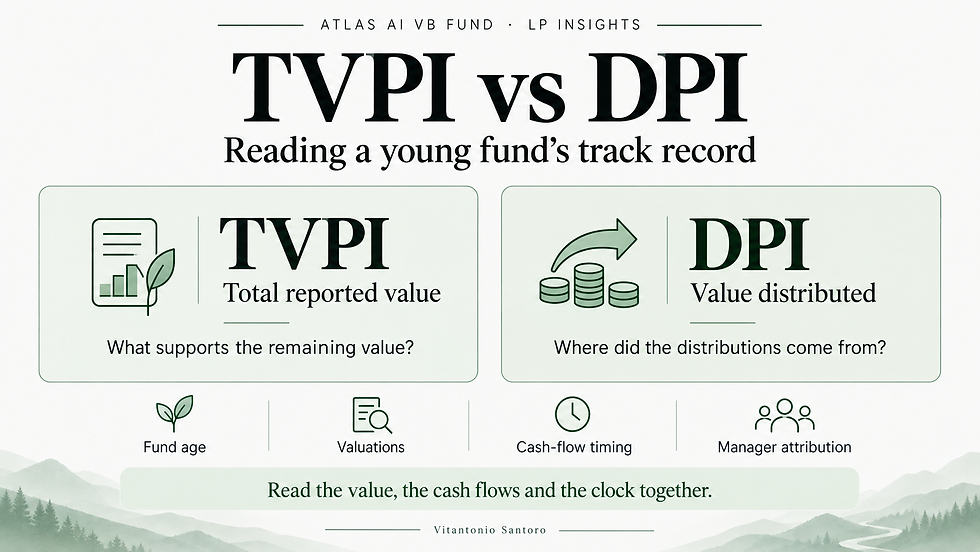
Carta’s Q1 2026 fund report reinforces the distinction: fewer than 20% of funds across its 2017 and 2018 cohorts had reached 1x DPI. The sample does not predict the timing of an individual fund. It makes a purely valuation-based return case insufficient. I discuss that distinction further in TVPI vs DPI: How to Read a Young Fund’s Track Record.
A stress test after the benchmarks
The reported data anchors the inputs. A scenario then makes the remaining assumptions visible. It should not be presented as the expected distribution of investment outcomes.
For the hypothetical €30 million fund, assume 40 investments averaging €607,500 each and no follow-ons, deploying the €24.3 million derived above. The following scenarios use final cash multiples on each investment, after dilution and company-level payout effects, but before fund fees and carry. Every company is fully realised; there is no remaining NAV.
Outcome or metric | Downside | One breakout | Larger winners |
|---|---|---|---|
Companies returning 0x | 28 | 24 | 20 |
Companies returning 1x | 8 | 8 | 8 |
Companies returning 3x | 3 | 6 | 8 |
Companies returning 10x | 1 | 1 | 3 |
Additional exceptional company | None | 1 at 50x | 1 at 100x |
Total companies | 40 | 40 | 40 |
Portfolio cash proceeds | €16.40m | €52.25m | €98.42m |
Gross investment multiple on €24.3m | 0.68x | 2.15x | 4.05x |
Final net distributions on €30m paid in | 0.55x | 1.59x | 2.82x |
The 0x, 10x, 50x and 100x counts are constructed stress tests, not observed portfolio frequencies or an empirical failure-rate forecast. The carry rate follows Carta’s reported median; the simplified distribution rules below remain assumptions. The last row assumes all €30 million is called, €5.7 million is spent on fees and expenses, and 20% carry is charged only on aggregate proceeds above the full €30 million contributed. There is no preferred return, catch-up, recycling, fund borrowing or additional tax leakage. Investors share the same economics.
The last scenario includes a 100x investment and three 10x investments, yet the final net multiple remains below 3x. Half the companies return nothing, and investment profits must absorb the fund’s costs before being shared with the manager.
Under these assumptions, distributing €90 million net to investors requires €105 million of portfolio proceeds: €30 million returned capital plus 80% of €75 million profit. That is a approximately 4.32x gross multiple on the €24.3 million invested.
This is why a gross portfolio multiple and an LP’s return need separate labels and denominators. The ILPA Performance Template distinguishes fund-level and portfolio-level performance and their cash flows. The simplified waterfall above is an illustration, not an ILPA reporting methodology or a substitute for a fund’s actual distribution terms.
The questions I would bring to an LP meeting
At Atlas AI VB Fund, our public thesis focuses on defensible AI at pre-seed and seed, sourced through venture builders and founder programs. That thesis needs to translate into attainable allocations, disciplined entry economics and financing paths that fit the fund. The investment manifesto explains the strategy; portfolio construction tests its economic implications.
I would want the discussion to resolve six questions:
How much committed capital can be invested after the full cost budget?
What ownership can the manager actually acquire at the prices and allocations available?
What remains after financing rounds, option pools and the exit payout terms?
How many large outcomes are required, and what happens if the largest never arrives?
What evidence supports the reserve policy and the opportunities it gives up?
When could proceeds reach LPs, and how does the result change if that takes longer?
For a manager raising a larger successor fund, I would add one more: which part of the strategy changes with the additional capital, and what evidence supports the ability to execute it?
My view is that portfolio construction earns an LP’s confidence when the manager can explain both the attractive outcome and the conditions under which it fails. The useful model connects the investment decision made today to the ownership, costs and cash flows that the investor may ultimately receive.
To discuss venture capital portfolio construction and the Atlas investment approach, contact Vitantonio Santoro.
About the author: Vitantonio Santoro is a General Partner at Atlas AI VB Fund.
This article is for general information and is not an offer to invest. The hypothetical scenarios do not represent expected or historical Atlas performance.

Comments